Dispersion Imaging Scheme (Passive Remote MASW)
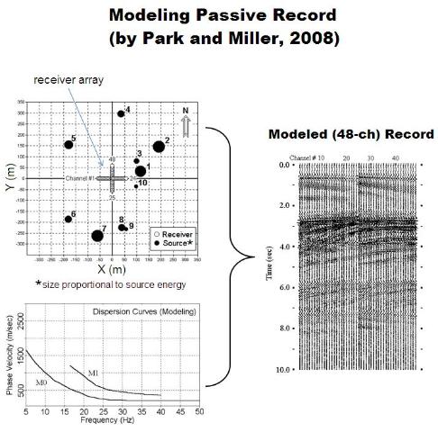
To explain the dispersion imaging scheme by Park et al. (2004), a 48-channel synthetic
record of passive surface waves is used that was generated according to Park and
Miller (2005) by considering arbitrary source points around a 2-D (cross) receiver array
with different source intensities (Fig. 1). This (modeled) field record has three
independent variables, two for the source coordinate (x and y) and one for time (t), to be
denoted as r (x, y, t). Then, FFT is applied to the time axis: R(x, y, w)=FFT[r(x, y, t)],
where w denotes the angular frequency.
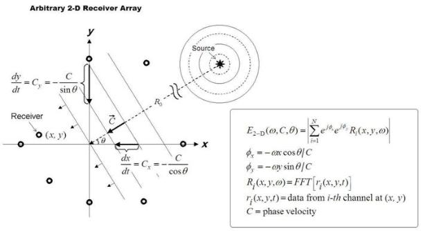
Then, for each frequency component within the analyzing range, energy corresponding
to a given azimuth angle for a given phase velocity is calculated according to the
projection principle illustrated in Fig. 2. This is repeated for different azimuths and
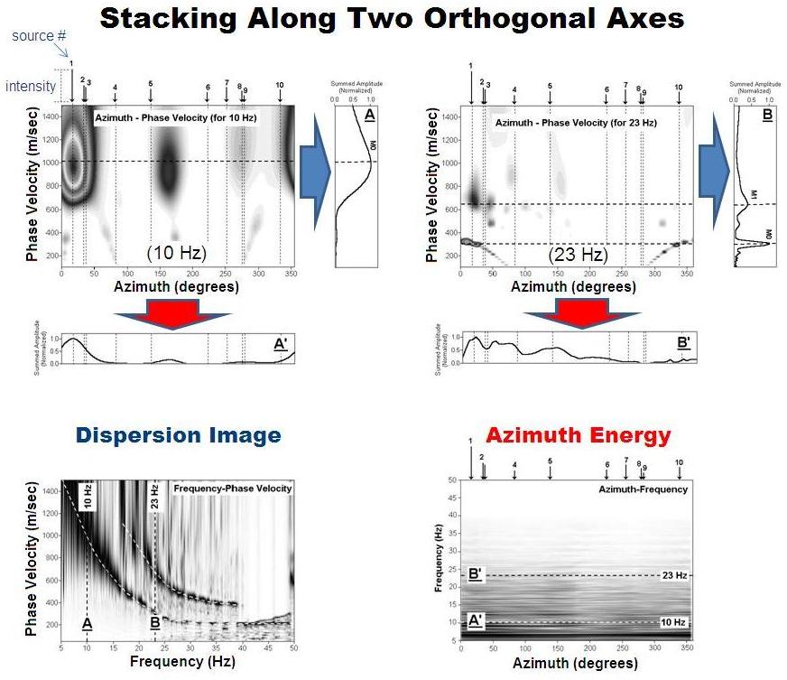
phase velocities within the analysis range of the two variables (e.g., 5-50 Hz with 0.1-Hz
increments and 10 m/sec-2000 m/sec with 5 m/sec increments ) to construct an
azimuth-energy mapping for one given frequency. Fig. 3 shows two of these maps
calculated for two arbitrary frequencies of 10 Hz and 23 Hz, respectively. In this map,
azimuths and phase velocities of those passive surface wave events recorded are
recognized from the energy peaks with peak height being proportional to the relative
source intensity. Peaks aligned in the azimuth-axis direction indicate the same mode
(as depicted from the same phase velocity) generated from different locations (as
depicted from different azimuths), whereas those aligned in the phase-velocity-axis
indicate different modes generated from the same location (Fig. 3).
Next, all the energy in each mapping is summed (or stacked) together along the
azimuth axis. The azimuth axis is then collapsed and only the phase velocity axis
remains where peaks indicate phase velocities of different modes for the frequency
being analyzed. This stacking has two advantages: 1) the same modes generated
from different locations (different azimuths) are constructively superimposed, and 2) all
the random energy peaks from computational artifacts and unrelated noise wavefields
are relatively suppressed.
To explain the dispersion imaging scheme by Park et al. (2004), a 48-channel synthetic
record of passive surface waves is used that was generated according to Park and
Miller (2005) by considering arbitrary source points around a 2-D (cross) receiver array
with different source intensities (Fig. 1). This (modeled) field record has three
independent variables, two for the source coordinate (x and y) and one for time (t), to be
denoted as r (x, y, t). Then, FFT is applied to the time axis: R(x, y, w)=FFT[r(x, y, t)],
where w denotes the angular frequency.
Then, for each frequency component within the analyzing range, energy corresponding
to a given azimuth angle for a given phase velocity is calculated according to the
projection principle illustrated in Fig. 2. This is repeated for different azimuths and
phase velocities within the analysis range of the two variables (e.g., 5-50 Hz with 0.1-Hz
increments and 10 m/sec-2000 m/sec with 5 m/sec increments ) to construct an
azimuth-energy mapping for one given frequency. Fig. 3 shows two of these maps
calculated for two arbitrary frequencies of 10 Hz and 23 Hz, respectively. In this map,
azimuths and phase velocities of those passive surface wave events recorded are
recognized from the energy peaks with peak height being proportional to the relative
source intensity. Peaks aligned in the azimuth-axis direction indicate the same mode
(as depicted from the same phase velocity) generated from different locations (as
depicted from different azimuths), whereas those aligned in the phase-velocity-axis
indicate different modes generated from the same location (Fig. 3).
Next, all the energy in each mapping is summed (or stacked) together along the
azimuth axis. The azimuth axis is then collapsed and only the phase velocity axis
remains where peaks indicate phase velocities of different modes for the frequency
being analyzed. This stacking has two advantages: 1) the same modes generated
from different locations (different azimuths) are constructively superimposed, and 2) all
the random energy peaks from computational artifacts and unrelated noise wavefields
are relatively suppressed.
All these steps are repeated for different frequencies. Gathering
of these stacked (summed) curves in the order of frequency will
constitute an energy field in two orthogonal axes of phase
velocity and frequency where dispersion trends are recognized
through the energy accumulation patterns (Fig. 3).
While the stacking energy in the azimuth-phase velocity space
along the azimuth axis results in dispersion images, the
stacking along the other axis (phase velocity) gives another
useful mapping, called azimuth-frequency space, that shows
energy distribution for different azimuths and frequencies (Fig. 3).
Comparing to the conventional wavenumber (f-k) method, the
azimuth scanning approach is more robust and straightforward
(Fig. 4).
(Right) Fig. 1. A sample modeling with a 48-channel cross receiver array and ten different source points of different intensities scattered around the array. Two dispersion modes are
incorporated in the modeling to generate the 10-sec long field record.
incorporated in the modeling to generate the 10-sec long field record.
(Right) Fig. 2. Projection principle to derive x- and y-components
of phase velocities for a surface wave arriving at angle of theta
with a phase velocity of C.
(Below) Fig. 3. Azimuth energy mappings for two arbitrary
frequencies of 10 Hz and 23 Hz, respectively and their stacked
energy along the two orthogonal axes leading to the dispersion
image and azimuth energy spaces.
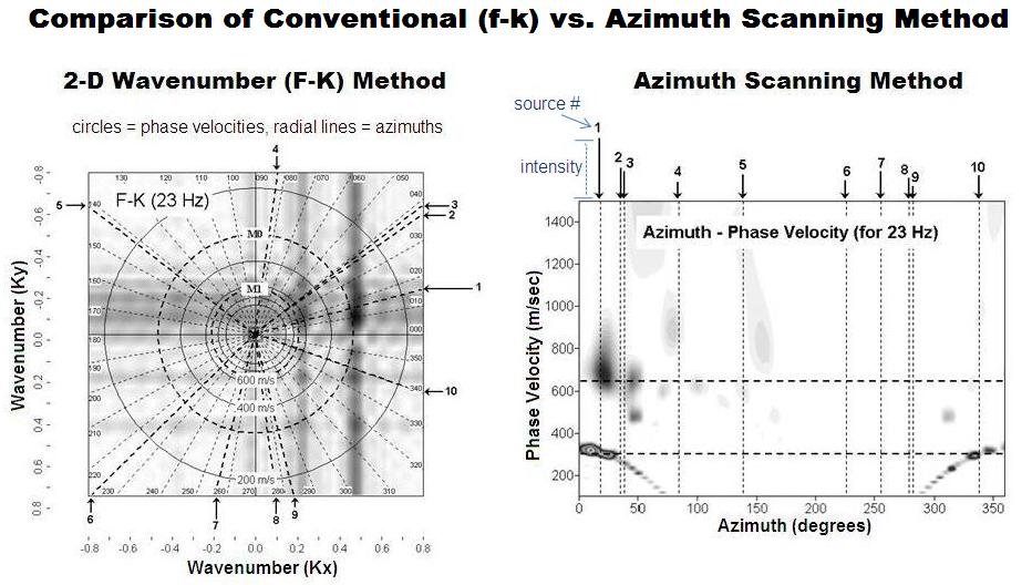
(Below) Fig. 4. Comparison of the conventional wavenumber (f-k) method and the azimuth scanning method, which is the foundation for the dispersion imaging scheme
described above.
described above.
| e-mail: contact@masw.com |
| | | | | | | | |