| e-mail: contact@masw.com |
| | | | | |
Product from MASW Surveys
Final product from an MASW survey is the subsurface variation of shear-wave velocity (Vs) in 1-D
(depth) (Figure 1), 2-D (depth and one surface direction) (Figure 2), and 3-D (depth and two
surface directions) (Figures 3 and 4) formats. The shear-wave velocity (Vs) most closely
represents stiffness of materials: the key property of all geotechnical engineering projects.
For 1-D survey, a receiver array is placed on the ground centered at a specific surface location
where a depth variation of subsurface velocity (Vs) is being investigated. In theory, only one field
record obtained with one source offset (X1) is sufficient to generate the 1-D velocity (Vs) profile.
In reality, however, multiple records with different source offsets (and also from both ends of
receiver array) are often used to minimize those possible adverse influences such as near- and
far-field effects and lateral variation of subsurface velocities. When the subsurface condition is
expected to be laterally homogeneous, then only one field record obtained with an optimum
source offset (usually about 25-50% of receiver array length) can be used for subsequent data
analysis to generate the 1-D profile.
Because all surface-wave methods, in theory, are based on a layered earth model, the data
analysis steps inevitably apply lateral averaging of subsurface conditions along the surface
distance occupied by the receiver array. As a result, the final 1-D profile can best represent the
subsurface velocity (Vs) model below the center of the receiver array as illustrated in Figure 1.
For example, the profile can be a 100% subsurface velocity (Vs) representation at surface
location of station 1050 in Figure 1, while it may represent less than 50% of subsurface model at
station 1045.
For a 2-D survey, the 1-D survey is basically repeated at successive locations along a preset
survey line (Figure 2). This will generate accordingly many 1-D velocity (Vs) profiles representing
subsurface velocity (Vs) models below successive surface locations. A simple 2-D interpolation
scheme (e.g., bilinear) is usually used to generate a 2-D velocity (Vs) grid-data set that in turn is
used to construct a 2-D cross section in which velocities are usually represented with different
color codes (Figure 2).
For a 3-D survey, the 2-D survey is repeated either in parallel or in perpendicular to each other
(Figure 3). Then, multiple 2-D velocity (Vs) data sets are used to make a 3-D (cubic) grid-data
set by using a 3-D interpolation scheme (e.g., tri-linear). There can be various ways to visually
present velocity (Vs) distribution by using a cubic grid. For example, slice maps (cross sections)
can be displayed along any specific direction of all three axes: depth (Z), West-East (W-E), and
South-North (S-N) (Figure 4). A bedrock topography map can also be constructed from multiple
2-D velocity (Vs) cross sections (Figure 5).
Because 2-D and 3-D surveys are basically repetitions of 1-D surveys at multiple locations, all
MASW surveys are 1-D surveys in theory.
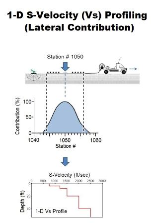
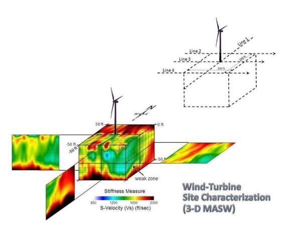
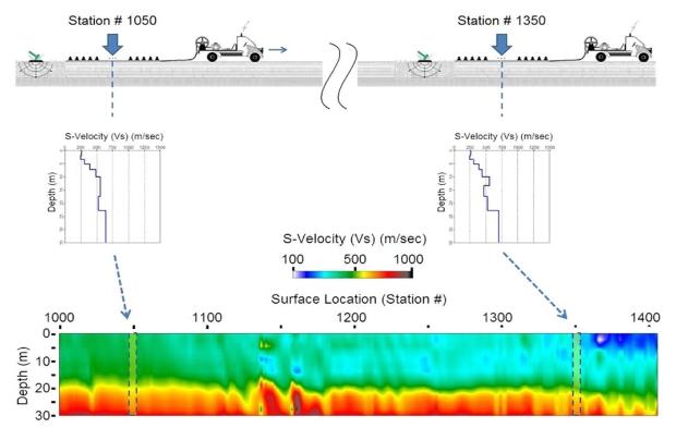
Figure 1. A schematic showing a field layout for
1-D MASW survey (top) and its final product of
S-velocity (Vs) profile (bottom). A curve is shown
that represents relative contribution of subsurface
velocity model at different lateral part within the
receiver array used for data acquisition (middle).
1-D MASW survey (top) and its final product of
S-velocity (Vs) profile (bottom). A curve is shown
that represents relative contribution of subsurface
velocity model at different lateral part within the
receiver array used for data acquisition (middle).
Figure 2. (left) A schematic showing field acquisition
procedure for 2-D MASW survey. A multichannel
field record obtained at one surface location (top)
generates one 1-D S-velocity (Vs) profile (middle),
multiple of which construct the final 2-D velocity (Vs)
cross section (bottom).
procedure for 2-D MASW survey. A multichannel
field record obtained at one surface location (top)
generates one 1-D S-velocity (Vs) profile (middle),
multiple of which construct the final 2-D velocity (Vs)
cross section (bottom).

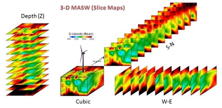
Figure 3. (right) A schematic showing field
acquisition procedure for 3-D MASW survey. Multiple
2-D surveys (e.g., Lines 1-4) run either in parallel or in
perpendicular generate multiple 2-D velocity (Vs)
cross sections that are used to generate a 3-D cubic
data set.
Figure 4. (below right) The 3-D data, once
constructed, can be used in various ways to visually
present velocity (Vs) distribution, one of which is
illustrated here for slice maps along three orthogonal
axes; i.e., depth (Z), West-East (W-E), and South-North
(S-N) axes.
Figure 5. (below left) A bedrock topography map
constructed from four (4) 2-D Vs maps at a proposed
wind-turbine site. An arbitrary and relatively high Vs
value of 1500 ft/sec was chosen to present the
soil/bedrock boundary.
| 1-D MASW |
| 2-D MASW |
| 3-D MASW |